As an accountant and former student, I have been using Excel for many years, but recently I’ve discovered some Excel tips that I find particularly useful when I’m on a tight deadline. From searching through the entire workbook for a reference error to adding a hyperlink to the summary tab, there are many ways to maximize your productivity with Excel.
1. Search Through Entire Workbook
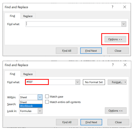
When you want to search for a particular word or number in one worksheet, “Ctrl + F” is usually the way to go. But if you click the “Options” button, you can choose to search through the entire workbook. This is very useful when you have multiple worksheets. For example, if you want to find all reference errors in your workbook and fix them all at once, you can enter “#REF” and then select “Formulas” in the dropdown box.
2. Copy Paste Only Visible Cells
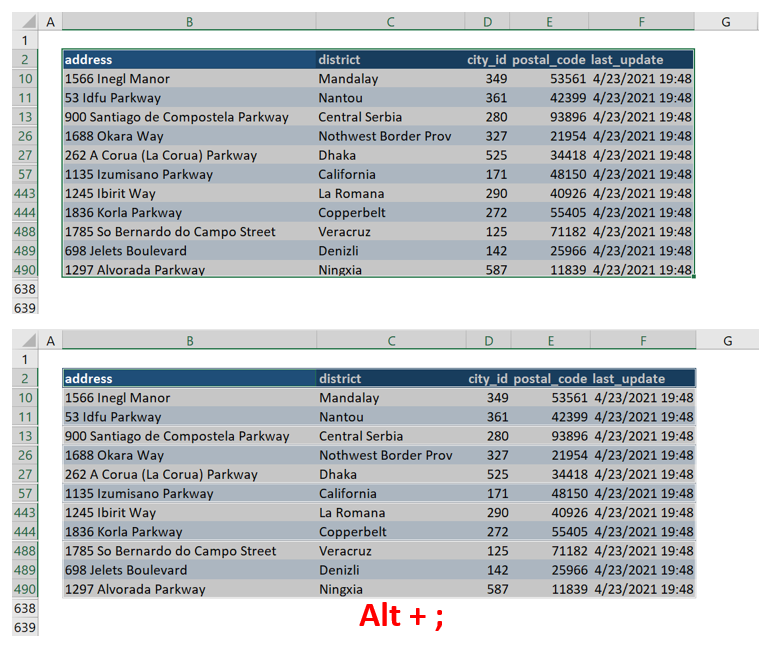
We sometimes need to hide certain rows and columns in Excel just like in the following table: it only shows the first couple of rows and then jumps to row 443. The problem appears when we want to copy these rows and only paste these rows. If we do regular “Ctrl + C” and “Ctrl + V”, all hidden rows will appear together with the visible rows. One way to address this issue is to highlight the table and then press “Alt + ;”, then do regular copying and pasting in Excel. This allows you to copy only the visible cells.
3. SUMPRODUCT
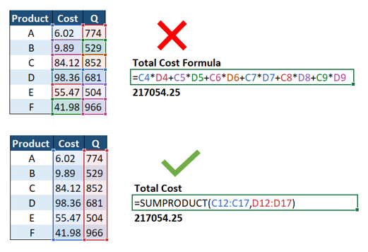
In the past, if I wanted to know the total cost of all products, I would have to multiply and add one-by-one. But now, thanks to “SUMPRODUCT”, I can just enter “=SUMPRODUCT” in the cell, and then select all costs, enter a comma, and then select all quantities. The total cost is calculated in a much clearer way.
4. HLOOKUP
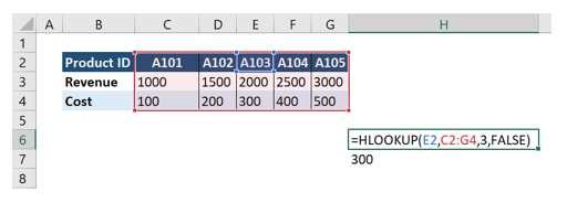
If your unique lookup value is listed in a row, you can use “HLOOKUP” to obtain all other information corresponding to that lookup value. For example, if you want to know the cost of the product ID “A103”. After you enter “=HLOOKUP” in a cell, you will be instructed to enter the lookup value, lookup table, relative position of the item you want to get, and the exact/approximate (FALSE/TRUE) match. In this case, the lookup value is “A103”; the lookup table is in a range from C2 to G4, or everything in the red box below; and the relative position is 3, because “Cost” is 3 cells away starting from the lookup value. In a real-world scenario, absolute reference and HLOOKUP are often used together.
5. VLOOKUP
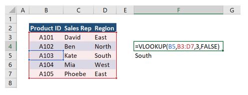
If your unique lookup value is listed in a column, you can use “VLOOKUP” to get all other information corresponding to that lookup value. For example, if you want to know the region of the product ID “A103”. After you enter “=VLOOKUP” in a cell, you will be instructed to enter the lookup value, lookup table, relative position of the item you want to get, and the exact/approximate (FALSE/TRUE) match. In this case, the lookup value is “A103”; the lookup table is in a range from B3 to D7, or everything in the red box below; and the relative position is 3, because “Region” is 3 cells away from the lookup value, starting from the Product ID column. In a real-world scenario, absolute reference and VLOOKUP are often used together.
6. Convert Table to Range
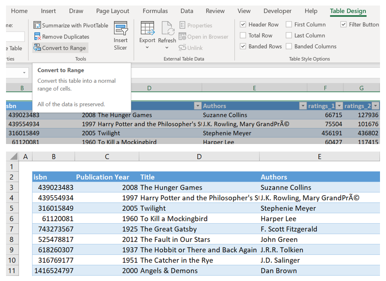
There are many functions that come along with the “Table” that you may not need. As such, you can remove all unnecessary functions but still keep the table style by converting it into a range. For example, once you click the “Table”, a “Table Design” tab will appear. Then, you can click “Convert to Range” under the “Tools” section to make it a regular range.
7. Group Data
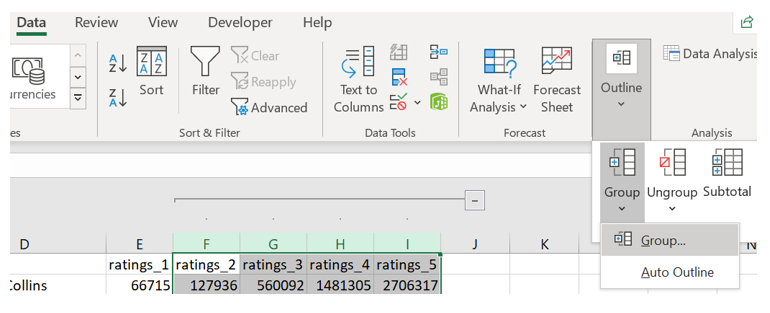
To make the Excel worksheet more organized and less intense for users, we can use the “Group” function under the “Outline” button listed on the “Data” tab. For example, if we have many different sections, we can collapse each section and only show the title of each section. This way, users can expand or collapse according to their preference.
8. Add Hyperlink to Summary Tab
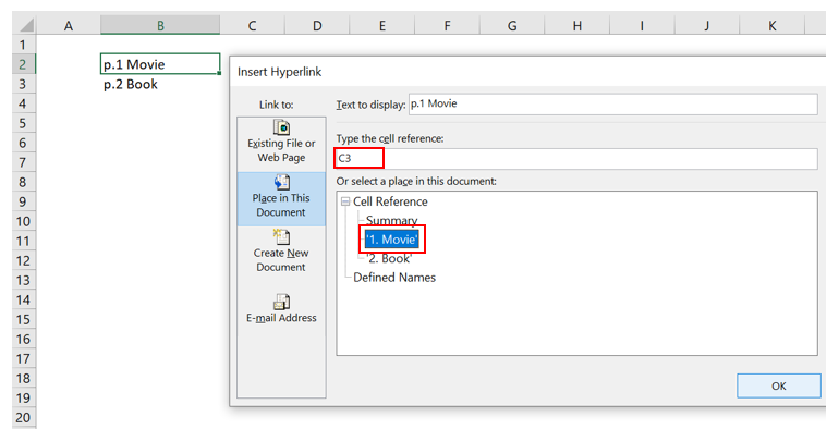
It’s always helpful to have a summary tab, which acts as a table of contents for your workbook. Each item in the table of contents can direct users to the specified tab through a hyperlink. You can select the cell you want to add a hyperlink. Then, by pressing “Ctrl + K”, the following dialog box appears. You can select “Place in This Document” under the “Link to”, and it will show all tabs you have in this workbook. Then, you can select a tab and type the cell you want to direct the user to under “Type the cell reference.”
9. Highlight Row or Column
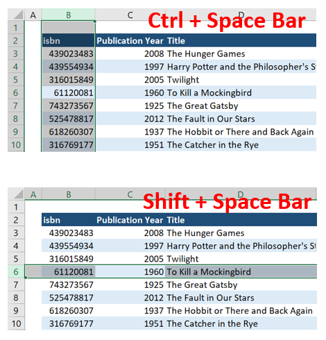
You can highlight a column by pressing “Ctrl + Space Bar” and highlight a row by pressing “Shift + Space Bar.”
10. Alternative Way of “Merge & Center”
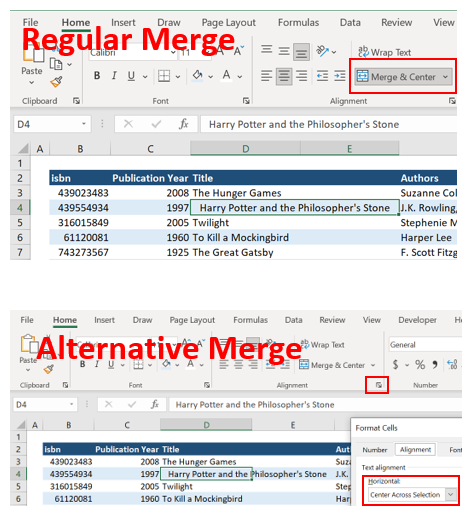
We often need to merge cells for titles or to accommodate other cells. As such, “Merge & Center'' has been used widely, but sometimes it creates issues when we do copy and pasting. A better solution to that is “Center Across Selection” in the “Alignment” section. It looks like we used “Merge & Center,” but it doesn’t create any issue when we do copy and pasting.
11. Find and Replace – Formatting
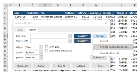
Previously, we mentioned “Find and Replace,” but it has another powerful function—replacing a certain cell’s (or cells’) formatting. You can choose an existing cell’s format and replace it with the format you want. I found this very useful when wanting to change many cells’ format at once.
12. Remove Gridlines and Leave White Space
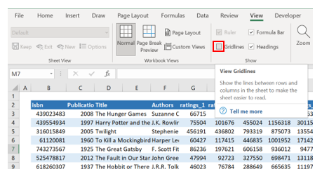
Removing gridlines makes your table easy to read. You can do this by unchecking “Gridlines” under the “View” tab. Additionally, it’s always better to leave some white space, like in the screenshot below. The table starts from cell “B2” instead of cell “A1” so that there is white space around the table.
These are just a few easy-to-use Excel tips to start off with. If you’re interested in learning more Excel tips and tricks, below are some Excel YouTube channels to help you go deeper:
ExcelIsFunTutorials Point (India) Ltd. - MS-Excel