Suppose you need to apply a filter on a column and paste each filtered table into a separate Excel sheet until all unique values have been filtered and pasted.This can be a very time-consuming process, especially if there are many rows on the Excel master sheet. However, it can be easily and quickly completed using Excel VBA. In this article, I will explain how to use VBA to divide data from the master sheet into separate Excel sheets based on the different filtered values. For demonstration purposes, I will be using Athletes dataset from Kaggle that contains all the athletes from the 2021 Japan Olympics. The steps are as follows:
Step 1. Create a List of Unique Values
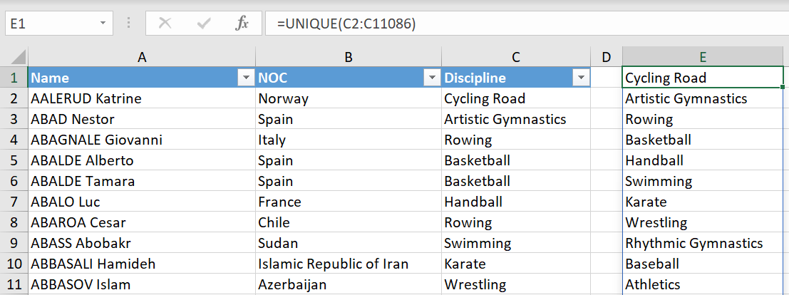
Find an empty column and type “=UNIQUE” in an empty cell. Then, select the entire column that will be filtered. Next, press “Shift + Enter.” This way, you will have a list of unique values from the column that will be filtered. I used column E as my empty column to list all the unique values from the “Discipline” column which will be filtered.

Step 2. Write VBA Code
You can find the “Developer” tab on the top ribbon of Excel. On the “Developer” tab, you can find “Visual Basic.” Once you click “Visual Basic,” there will be a drop-down menu on the top left of the new screen where you can find “Module.” Once you click this, it opens the VBA editor. Alternatively, you can press “Alt + F11” to open the VBA editor. Then, you can write the following code in the VBA editor:
Sub FilterSeperateIntoTabs()

'Declare all the variables
Dim currRow As Integer
Dim i As Integer
Dim Names As String

'Use a “while loop” to loop through unique “Discipline names” that we generated in column E. Starting from the cell “E1.” For example, in the first loop, we get “Cycling Road” as the “Name”
i = 1
While Range("E" & i) <> ""
Range("E" & i).Activate
Names = Range("E" & i).Value

'Activate the mastersheet
Sheets("Mastersheet").Activate

'Apply filter to the table. Our filtered column is the third one counting from the left, which is why the Field is equal to 3 and criteria is based on the “Name” we obtained above. In this case, Name, in the First loop is “Cycling Road”.
ActiveSheet.Range("C1").AutoFilter _
Field:=3, _
Criteria1:=Names, _
VisibleDropDown:=True

'Once filter is applied based on “Cycling Road”, we should get the last row number of the filtered table
currRow = Range("A1").End(xlDown).Row

'Copy the range specified below
Range(Cells(1, "A"), Cells(currRow, "C")).Copy

'Add a new sheet with the name “Cycling Road” during the first loop
Sheets.Add(, After:=Sheets("Mastersheet")).Name = Names

'Paste the data, auto adjust the column width, and select the cell “A1”
Range("A1").PasteSpecial (xlPasteAllUsingSourceTheme)
Range("A:C").EntireColumn.AutoFit
Range("A1").Select

'Go back to the mastersheet and activate it
Sheets("Mastersheet").Activate

'Unfilter the table
If ActiveSheet.FilterMode = True Then
Sheets("Mastersheet").ShowAllData
End If

'Increment i, so we can start our second loop and filter by “Artistic Gymnastics”. It will repeat the same steps listed above, starting from While Range("E" & i) <> ""
i = i + 1

'Once the condition Range("E" & i) <> "" in the while loop becomes false, we exit our loop
Wend

'End program
End Sub
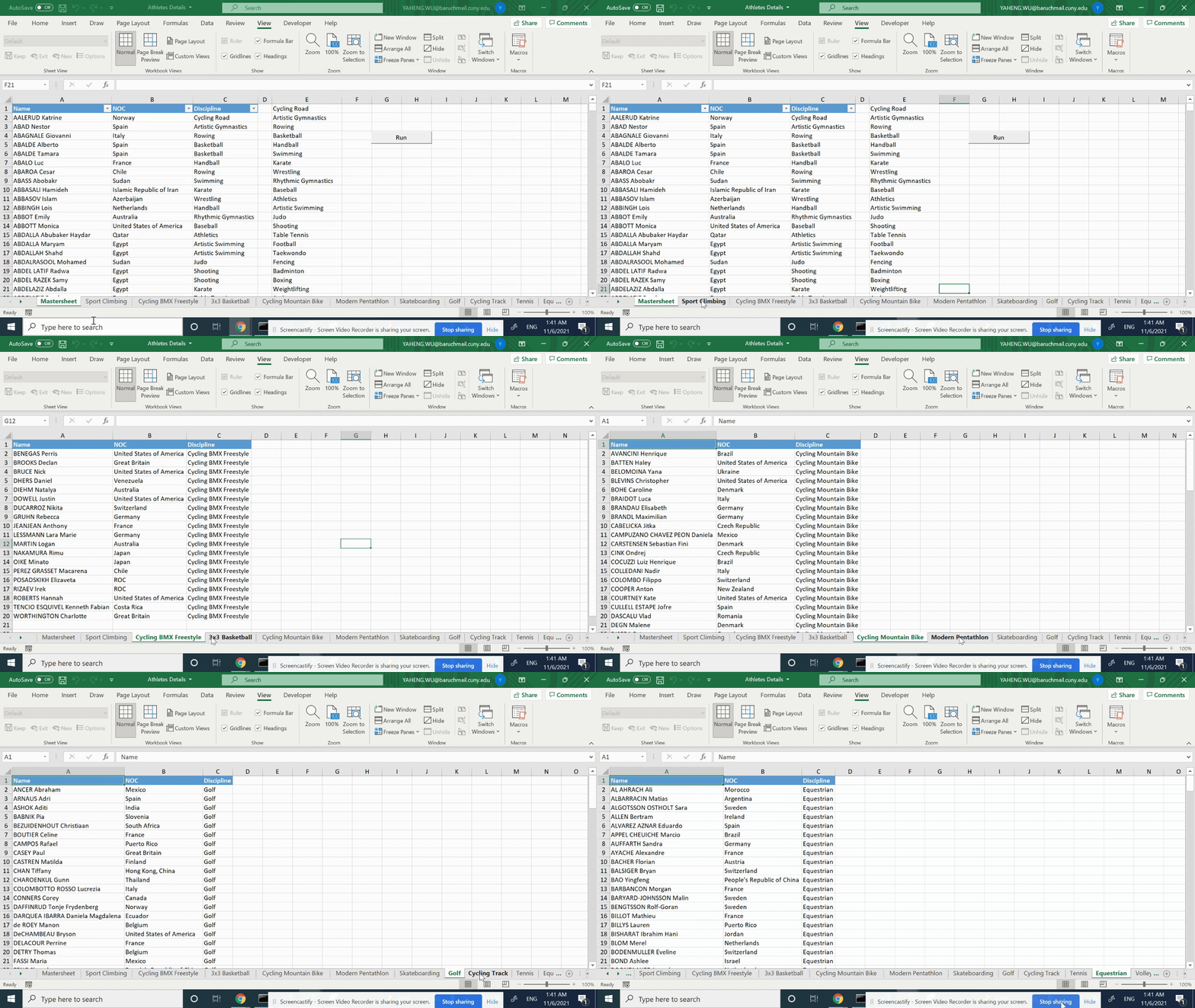
The result of the code above looks like this:

You can copy the code above and try it yourself. But you should definitely endeavor to understand how the code works so that you can apply it in any similar situation.